Quantile Regression for Weather Risk Pricing

I built the ML components for a weather prediction market (CS 506 team project): models that generate risk-adjusted odds for temperature, wind speed, and precipitation outcomes.

Ensembles require uncorrelated errors

I started with an averaging ensemble of XGBoost, RandomForest, and LightGBM. The first implementation hit a feature count mismatch at inference (82 vs 73 features) because feature lists were defined locally in training scripts rather than serialized with the models.

After centralizing feature definitions, the ensemble achieved 5.00°F MAE -- identical to XGBoost alone. All three are gradient boosting variants trained on the same features. They fail on the same inputs, so averaging adds nothing.

Stacking with a Ridge meta-model confirmed this: weights of 0.55 (XGBoost), 0.42 (LightGBM), 0.03 (RandomForest). Introducing algorithmic diversity (Ridge, SVR, MLP alongside XGBoost) didn't help either; the meta-model assigned 80% weight to XGBoost. A single tuned model outperformed every ensemble configuration.

Point predictions to distributions

5.00°F MAE is a reasonable point forecast, but point predictions can't set odds. 77°F doesn't tell the platform whether that's a confident prediction or a volatile one. Pricing wagers requires the model to output a distribution, not a number.

XGBoost supports quantile regression natively via reg:quantileerror. I trained three models (P10, P50, P90) per target:

base_model = xgb.XGBRegressor(
    objective='reg:quantileerror',
    quantile_alpha=quantile,  # 0.1, 0.5, or 0.9
    random_state=RANDOM_SEED,
    n_jobs=-1,
    tree_method='hist'
)

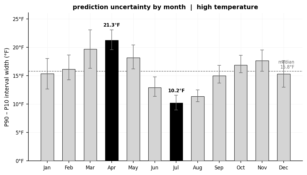
The P10/P90 outputs define an 80% prediction interval. The spread (P90 - P10) is the risk signal: 4°F means tight odds, 9°F means the house widens its margin.

Feature engineering produced 90 candidates -- cyclical temporal encodings, rolling windows (3/7/14/30-day), lag features, meteorological interactions. RFECV reduced that to 11-16 per target. Hyperparameter tuning used Optuna with TimeSeriesSplit to avoid temporal leakage. The pipeline serializes twelve artifacts: one feature selector and three quantile models per target.

Final MAE: 4.35°F on a held-out test set, down from 5.00°F.

Calibration

On the held-out set, P10-P90 intervals captured actuals 81-85% of the time across all three targets (nominal: 80%). Backtesting confirmed the house margin converges to the 10% target.

The intervals also track seasonal volatility: April averages 21°F wide, July averages 10°F.

I later ported this pipeline to CardinalCast, a standalone Python/FastAPI implementation.